My title

Author

Affiliation

My name

Simon Fraser University

Header 1

Header 2

Some text.

Formatting

Note that each header automatically creates an anchor, making it easy to link to specific sections of your documents.

Text can be rendered in italic or in bold as well as underlined.

You can use superscripts², subscripts_test, ~~strikethrough~~, and inline code.

This is a quote.

Columns

You can create columns.

And you can set their respective width.

Lists

Item 1
Item 2
Item 3

Ordered lists

Item 1
Item 2
Item 3

Images

Tables

Col 1	Col 2	Col 3
a	1	red
b	2	orange
c	3	yellow

Note

Tables can be fully customized (or you could use raw html).

Equations

\[ \frac{\partial \mathrm C}{ \partial \mathrm t } + \frac{1}{2}\sigma^{2} \mathrm S^{2} \frac{\partial^{2} \mathrm C}{\partial \mathrm C^2} + \mathrm r \mathrm S \frac{\partial \mathrm C}{\partial \mathrm S}\ = \mathrm r \mathrm C \]

Cross-references

See Section 1.2.

Note that you can add bibliographies, flow charts, the equivalent of HTML “div”, and just so much more. Remember that this is a tiny overview.

Let’s try some code blocks now

# This is a block that runs
2 + 3

[1] 5

Did you notice that the content of your code blocks can be copied with a click? Of course, this is customizable.

# This is a block that doesn't run
2 + 3

  country var
1  Canada 2.9
2     USA 3.1
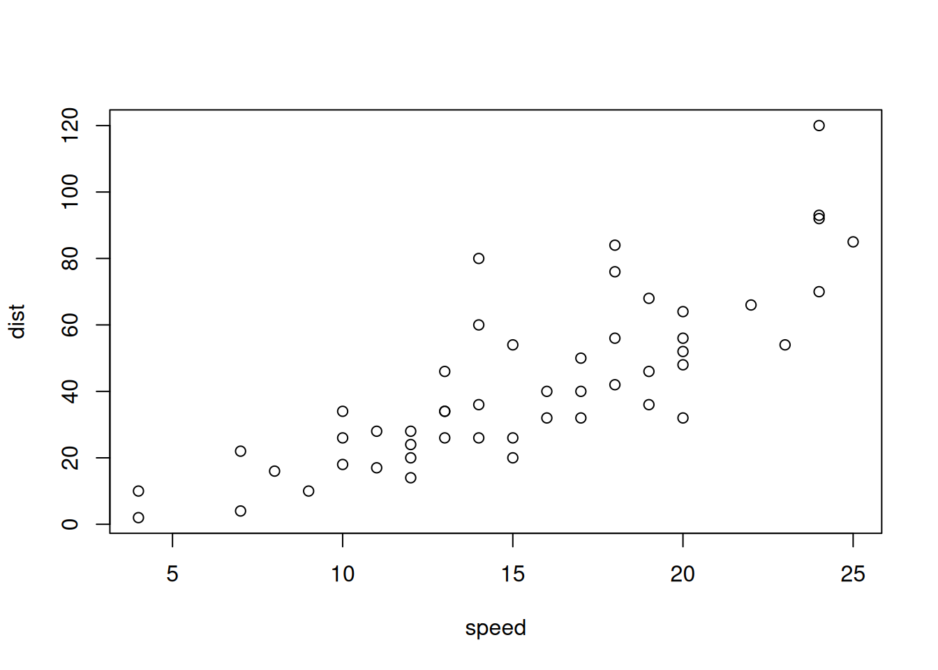
3  Mexico 4.5

Plots

plot(cars)

You can play with options to add a title:

plot(cars)

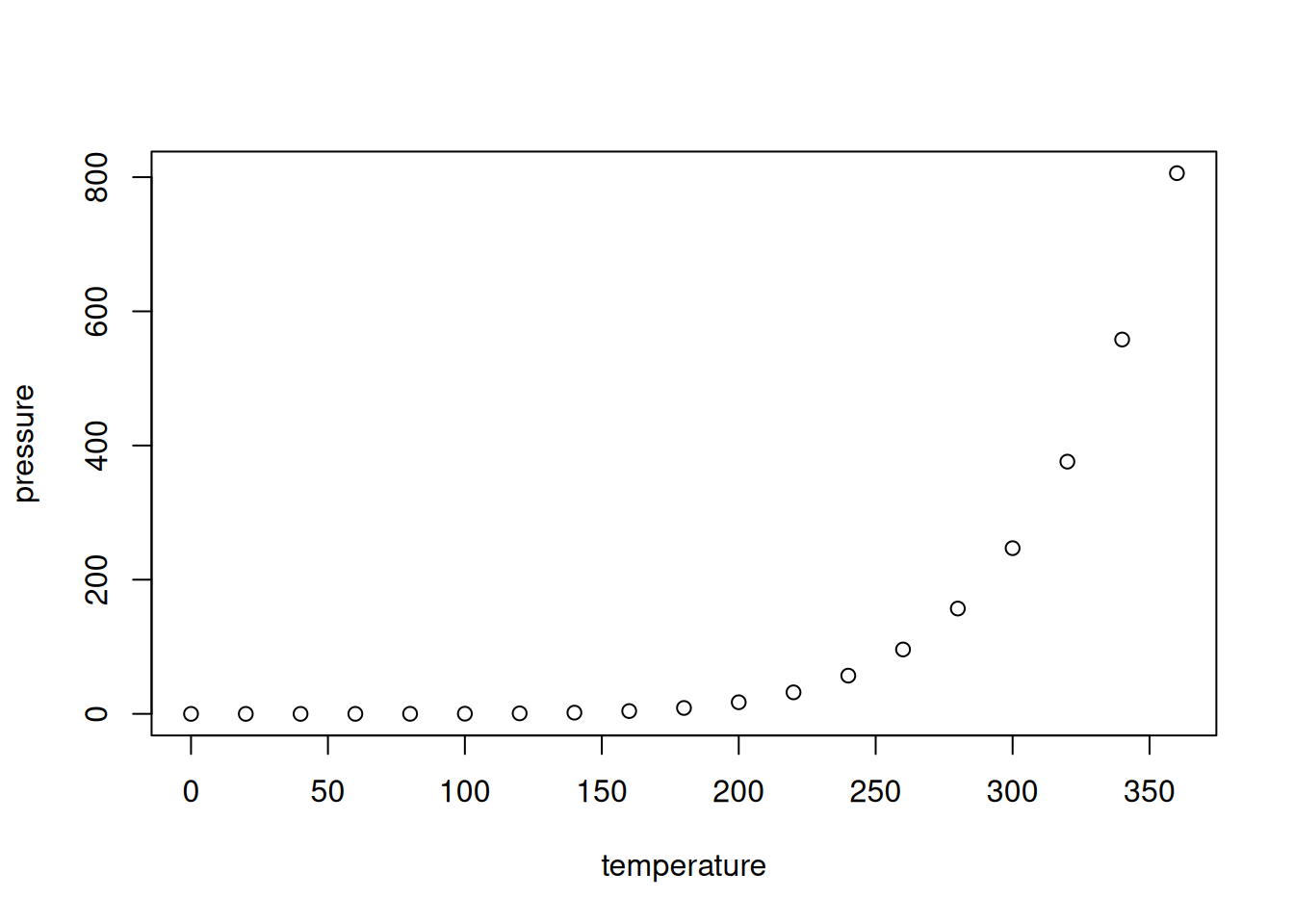
Stopping distance as a function of speed in cars

You can have more complex multi-plot layouts:

plot(cars)
plot(pressure)

Vapor pressure of mercury as a function of temperature

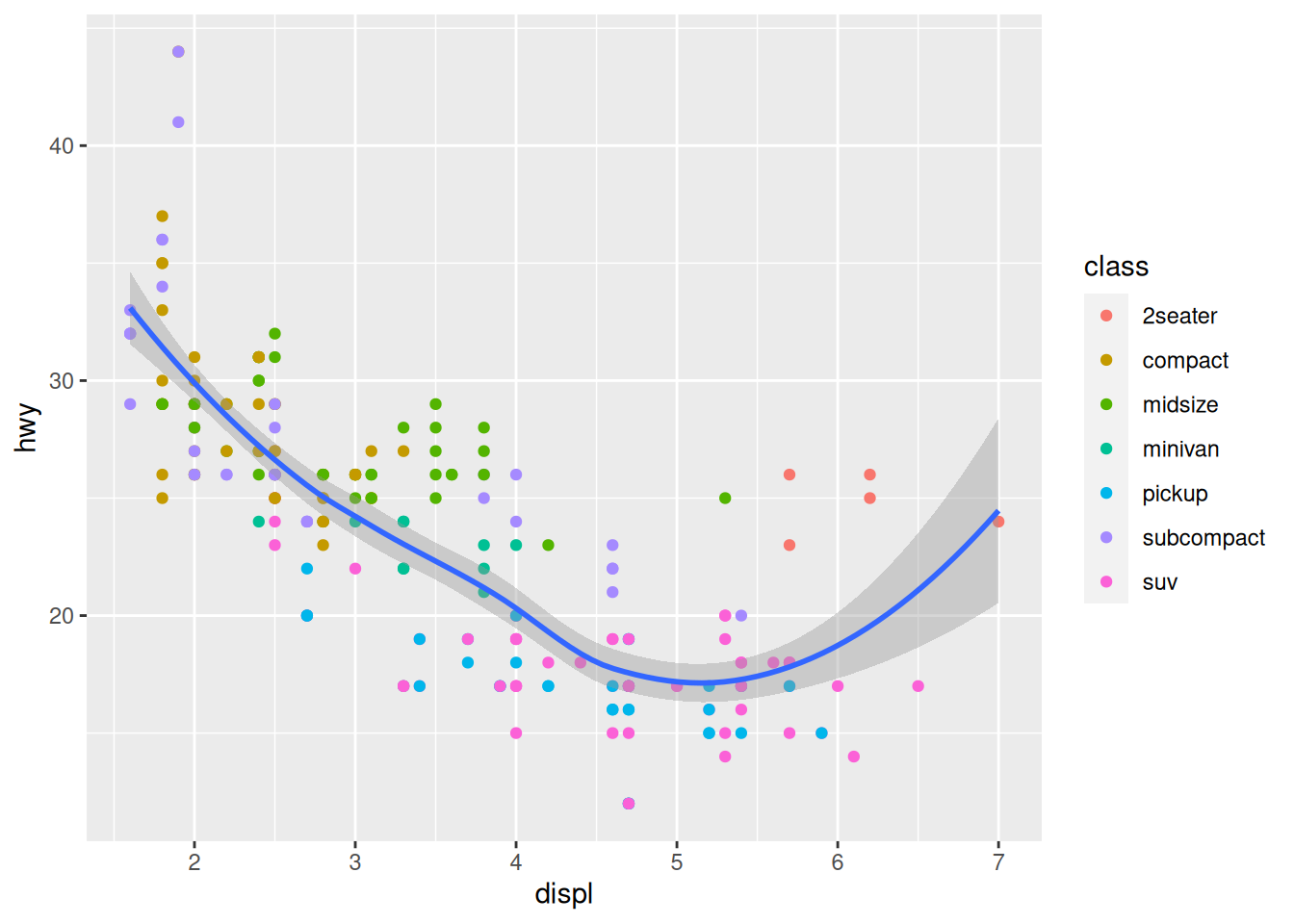
For those who have ggplot2¹, you can try that too:

library(ggplot2)

ggplot(data = mpg, mapping = aes(x = displ, y = hwy)) + 
  geom_point(mapping = aes(color = class)) + 
  geom_smooth()

`geom_smooth()` using method = 'loess' and formula = 'y ~ x'

Footnotes

You can install it with:
```
install.packages("ggplot2")
```
↩︎